Input form. Syntactically, a matrix is entered as a comma-separated list of
tuples delimited by brackets. An example matrix with 2 rows and three
columns is input as
[(0,1,2),(3,4,5)]
and displayed as
[(0, 1, 2), (3, 4, 5)]. The tuples that make up the rows need not be the same length.
However, shorter tuples are padded with zeroes to make all the rows
the same length in the matrix display.
There are some alternate input forms for special matrices.
The identity matrix is entered as [1] and displayed as ɪ.
The zero matrix is entered as [0] and displayed as [0].
Both conform to whatever size is required by the context in which
they appears.
Note the difference between [1] and [(1)]; the latter is a one-by-one matrix.
A column matrix is entered without row tuples: [1,2,3] is
[(, 1), (, 2), (, 3)].
Operations. Binary operators can be applied to matrices with the same
cardinality. If one operand is a scalar, it is promoted to a matrix.
Multiplication.
Matrix multiplication is performed by the multiplication operator, entered
using the scalar multiplication operator. The parser promotes the operator
to one appropriate to its operands. If
the left operand is a row vector, it is promoted to a one-row matrix. If
the right operand is a column vector, it is promoted to a one-column matrix.
That is,
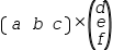
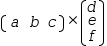
[(a, b, c)]×(d, e, f)ƈ
is treated like
[(a, b, c)]×[(, d), (, e), (, f)].
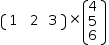
Note, however, the difference between [(1, 2, 3)]×[(, 4), (, 5), (, 6)]
and (1, 2, 3)ʋ∘(4, 5, 6)ƈ. The former produces a one-by-one matrix result
[(, 32)] while the latter produces a scalar result 32.
Concatenation. Matrices can be formed by concatenating two matrices, or by
concatenating a matrix with a tuple or a scalar. The operand with a
"lesser size" is expanded to conform to the operand with a larger size
by padding with zeros. Both horizontal and vertical concatenation are
supported using the binary ‖ and ‖‖ operators.
Horizontal concatenation displays as Mɱ‖Mɱ and vertical concatenation
displays as Mɱ‖‖Mɱ.
Take and Drop. Matrices can be partitioned using take and drop operators ↑ and ↓. These
are asymmetric binary operators that take a matrix on the left and a
specifier on the right to produce a matrix by extracting rows and
columns. The specifier is a real or tuple of reals. For take, the
number of rows and columns in the result is taken from the pair of
scalars in the tuple. If the right operand is a real it specifies rows and all the
columns are taken. If the right operand is a singleton tuple, the
single value specifies columns and all the rows are taken. Negative
values cause trailing rows or columns to be taken. If the magnitude of
a take specification is larger than the corresponding dimension of a
matrix, the result is padded with rows and columns of zeroes. Padding
in the form of rows or columns with zero-valued items is added to the
end of the result if the specification is positive and to the
beginning of the result if the specification is negative.
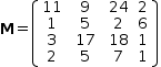
For example, the comatrix of a matrix element is another matrix
consisting of all the rows and columns of the containing matrix except
those containing the element. For matrix
Matrix Variable.
A matrix can be bound to a variable in a definition or associated with
a variable in an equation following the same rules as binding tuples.
When used in another expression, an explicit matrix variable can be
entered using a type suffix m or ɱ
[1].
Transpose.
The transpose operator, denoted by the unary postfix operator
T, can be applied to matrices and tuples. A transposed tuple is
transformed into a column matrix.
That is, [(a, b, c), (d, e, f)] T transforms to [(a, d), (b, e), (c, f)].
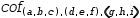
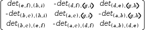
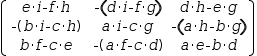
Cofactor. The cofactor operator, denoted by the unary postrix
operator
C
transforms a matrix by replacing each element by the determinant of
its cofactor matrix and using alternate signs.
That is,
Cardinality.
The
cardinality
operator is entered and displayed the same as for tuples. It produces
a real containing the number of rows. The number of columns can be
obtained using the column-cardinality operator, entered as as
#_1. Both forms display the same way.
#[(, 1), (, 2), (, 3)]
##[(, 1), (, 2), (, 3)]
(a) Row
(b) Column
Figure 6.1 Matrix cardinality
Special Simplification. Special simplification collapses a matrix to a tuple if all rows
are the same. It collapses a matrix to a scalar if it can be collapsed
to a row whose items are the same.
Row Echelon.
A matrix can be transformed to row-echelon form. If the matrix is
first concatenated on the right with the identity matrix, the right
half of the result represents the inverse after the row-echelon
transformation is applied. The inverse can also be produced by the
inverse operator, denoted by exponentiation with the power -1. That
is, the input
[(1,2),(3,4)]^-1
displays as
[(1, 2), (3, 4)]^-1
and simplifies to
[(, -2, 1), (3/2, -(1/2))]
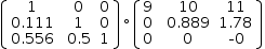
Factoring. A matrix can be factored into a
lower-diagonal matrix with ones on the diagonal and an upper-diagonal
matrix.
That is, [(1, 2, 3), (5, 6, 7), (9, 10, 11)] factors to
[(1, 0, 0), (0.1111111111111111, 1, 0), (0.5555555555555556, 0.5000000000000002, 1)]∘[(9, 10, 11), (0, 0.8888888888888888, 1.777777777777778), (0, 0, -8.881784197001252E-16)]
The matrix product of these two matrices is the same as the original matrix with some rearrangement of rows.